| Home | Contents | Start | Prev | 1 | 2 | Next |
Stochastic Processes
Up until this point, it has been possible to intuitively work out the possible locations where the robot is based on its sensor (and latterly, with movement) information. To realize this with deterministic logic in software is going to be a non-starter with a complex map, so we need to take a stochasitic approach and calculate the likelyhood that the robot is in a certain position, based on a probability distribution of all the locations in the map. This may not give black-and-white answers but we can always use a high probability as as our best estimate (eg if the probability of being in a grid cell > 0.85, then assume we are localized). It is computationally prohibitive to calculate every single move and remember its impact (like working out every combination in a chess game). A recursive mechanism where the current state is based on the previous state only is more realistic. This is a special kind of property called a Markov Chain.
When modelling the problem in software, we will need a map of the robot world in memory, as well as a model of where the robot thinks it is in relation to the real map. These are 'belief-states', namely each state represents the robots belief as to how probable it is to be in that state. For my initial investigations, there will be a 1:1 mapping between belief-states and robot-world states. On the grid diagrams, the belief-states will be overlayed on the robot-world grid (due to the 1:1 mapping).
The Starting Point - Prior Probability
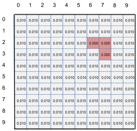
There are 100 grid cells. If three of these cells are 'blocked', that means there are 97 free locations. If the robot could be placed randomly, in any of the 97 free cells, then there is a uniform probability distribution that the robot can equally be in any of 97 locations. Assuming a zero probability of being in the 3 blocked states, this means the probability of being in any one free grid cell = 1/97 = 0.010. This is the prior probability - our starting estimate.
|
This is the starting state where the robot could randomly be in any of these positions. Each belief-state therefore has a probability of 0.010. This is prior to taking any sensor readings. The only thing we can be absolutely sure of is that we are not in states (2,6), (2,7) or (3,7) as the zero probability means we can never go there. |
So what now? If we take sensor readings, how can we use this to refine our belief states? This is where Bayes Theorem comes to the rescue. Bayes theorem can be stated:
P(A | B) = (P(B | A) * P(A))/P(B)
What this is saying is we can calculate the probability of A, given B if we know the probability of B given A. This is amazingly useful as we can turn a probability around. (eg instead of saying: "what is the probability of getting heads given I randomly chose a loaded coin", we instead say "what is the probability I chose a loaded coin given I got heads on a coin flip". The key is that choosing the coin randomly was non-observable, but the result of coin flip was, and from that we can deduce something about the non-observable coin selection.
All this directly applicable to robot localization. We cannot directly observe where we are to calculate the probability of our belief-state (equivalent to choosing a loaded coin from a bag at random). However, we can sense or observe obstacles (equivalent to seeing the result of the coin flip) and from these observations, we can infer our probability of being in a belief-state.
Sensing Simulation
A program was written to simulate the sensing mechanism by implementing Bayes Theorem. The robot-world map was defined so that the robot could move north, south, east or west by one square, provided the exit was not blocked.
This is the prior. I'm using integer arithmetic and probabilities are shown as a percentage, rounded down to the nearest whole number. We can see at the start that there is a 1% (probability = 0.0103) of the robot being in any square apart from the 3 blocked ones
 Prior:
1	1	1	1	1	1	1	1	1	1
1	1	1	1	1	1	1	1	1	1
1	1	1	1	1	1	0	0	1	1
1	1	1	1	1	1	1	0	1	1
1	1	1	1	1	1	1	1	1	1
1	1	1	1	1	1	1	1	1	1
1	1	1	1	1	1	1	1	1	1
1	1	1	1	1	1	1	1	1	1
1	1	1	1	1	1	1	1	1	1
1	1	1	1	1	1	1	1	1	1
Sense test 1
Starting with our prior and applying a sense of 'free to move in all 4 directions', we get the following result. We can see the probability distribution has changed so we know we are at none of the edge cells (cannot move 4 directions) and also the cells adjacent to the obstacle. The output shows 1% in the cells but this is actually a probability of 0.0185 (truncated) so our probability of being in those locations has increased.
Posterior:
0	0	0	0	0	0	0	0	0	0
0	1	1	1	1	1	0	0	1	0
0	1	1	1	1	0	0	0	0	0
0	1	1	1	1	1	0	0	0	0
0	1	1	1	1	1	1	0	1	0
0	1	1	1	1	1	1	1	1	0
0	1	1	1	1	1	1	1	1	0
0	1	1	1	1	1	1	1	1	0
0	1	1	1	1	1	1	1	1	0
0	0	0	0	0	0	0	0	0	0
Sense test 2
Lets try another sense reading. Starting with the original prior, lets assume our sensor says we can move in any direction apart from west, the west exit is blocked. Puting this into the simulation gives quite different results. We have narrowed down the possibility of localization to 10 states, just those that are blocked to the west, giving a 10% chance of being in any one of those states. Note this includes being blocked by the obstacle.
Posterior:
0	0	0	0	0	0	0	0	0	0
10	0	0	0	0	0	0	0	0	0
10	0	0	0	0	0	0	0	10	0
10	0	0	0	0	0	0	0	10	0
10	0	0	0	0	0	0	0	0	0
10	0	0	0	0	0	0	0	0	0
10	0	0	0	0	0	0	0	0	0
10	0	0	0	0	0	0	0	0	0
10	0	0	0	0	0	0	0	0	0
0	0	0	0	0	0	0	0	0	0
Sense test 3
Lets try another sense reading. Starting with the original prior, assume our sensor tells us exists are blocked to the north and east. The results tie up with the earlier intuitive reasoning, we have narrowed our belief states down to two, and have a 50% chance of being in either state.
Posterior:
0	0	0	0	0	0	0	0	0	50
0	0	0	0	0	0	0	0	0	0
0	0	0	0	0	0	0	0	0	0
0	0	0	0	0	0	50	0	0	0
0	0	0	0	0	0	0	0	0	0
0	0	0	0	0	0	0	0	0	0
0	0	0	0	0	0	0	0	0	0
0	0	0	0	0	0	0	0	0	0
0	0	0	0	0	0	0	0	0	0
0	0	0	0	0	0	0	0	0	0
So implementing Bayes Theorem based on sensor readings across the map does indeed produce the expected probability distribution. It helps reduce the belief states but this alone will not be sufficient to fully solve the localization problem. Earlier intuitive reasoning showed that moving the robot and then re-sensing would help minimize the number of belief states and so this was the next step.
Initially, lets assume the robot moves where we want it to, one grid cell at a time i.e. if we ask it to go north it will move one grid cell north and not go east, west or stay still. Given this assumption (and that is a big assumption), what would this do to the probability distribution? Well if the whole probability distribution moves with the robot, we could get some misleading results until we sense again. However, shifting the distribution keeps a record of the movement in the beilefs states. We are in a different position now so the sensor reading change and when we apply this to the probability distribution, we should be able to pare down the number of belief states. A repeated combination of sense-move steps should eventually lead us to a unique place on the grid and we will then be localized.
Sense and Move Test 1
Taking again, the sensor reading from senseTest1
Posterior:
0	0	0	0	0	0	0	0	0	0
10	0	0	0	0	0	0	0	0	0
10	0	0	0	0	0	0	0	10	0
10	0	0	0	0	0	0	0	10	0
10	0	0	0	0	0	0	0	0	0
10	0	0	0	0	0	0	0	0	0
10	0	0	0	0	0	0	0	0	0
10	0	0	0	0	0	0	0	0	0
10	0	0	0	0	0	0	0	0	0
0	0	0	0	0	0	0	0	0	0
Now if we apply move north, using the above distribution as our prior, then sense again (and find west is blocked), we see that two belief states have fallen away (probability -> 0) and we now have a 12% chance of being in any one of the 8 states.
Posterior:
0	0	0	0	0	0	0	0	0	0
12	0	0	0	0	0	0	0	0	0
12	0	0	0	0	0	0	0	12	0
12	0	0	0	0	0	0	0	0	0
12	0	0	0	0	0	0	0	0	0
12	0	0	0	0	0	0	0	0	0
12	0	0	0	0	0	0	0	0	0
12	0	0	0	0	0	0	0	0	0
0	0	0	0	0	0	0	0	0	0
0	0	0	0	0	0	0	0	0	0
We can continue this procedure and will eventually find we converge, provided the robot can find a unique state. For example, assume we had started in state (3,8). We have sensed and moved north once. If we move north again, in reality we should be in state (1,8). When we sense in this state, we should have no obstacles in any direction (unlike all the other belief states on the western wall, so we should localize. Here are the results of doing this:
Posterior (sense):
0	0	0	0	0	0	0	0	0	0
0	0	0	0	0	0	0	0	100	0
0	0	0	0	0	0	0	0	0	0
0	0	0	0	0	0	0	0	0	0
0	0	0	0	0	0	0	0	0	0
0	0	0	0	0	0	0	0	0	0
0	0	0	0	0	0	0	0	0	0
0	0	0	0	0	0	0	0	0	0
0	0	0	0	0	0	0	0	0	0
0	0	0	0	0	0	0	0	0	0
And we have localized.
Sense and Move Test 2
Lets try one more example, that of sensetest3. In this case, after the first sense, we had narrowed down our belief state to two (3,6) and (0,9). If we move west and then sense again, if the there is no blockage to the north, we are in state (3,5), otherwise we must be in state (0,8). Running the simulation yields:
Posterior (sense):
0	0	0	0	0	0	0	0	0	0
0	0	0	0	0	0	0	0	0	0
0	0	0	0	0	0	0	0	0	0
0	0	0	0	0	100	0	0	0	0
0	0	0	0	0	0	0	0	0	0
0	0	0	0	0	0	0	0	0	0
0	0	0	0	0	0	0	0	0	0
0	0	0	0	0	0	0	0	0	0
0	0	0	0	0	0	0	0	0	0
0	0	0	0	0	0	0	0	0	0
So the test results look very encouraging. Having a pre-defined map and some suitable distance sensors, a compass and not too many errors, then applying the sensor data to the map will go a long way to identifying where we are on the map. Moving around and re-sensing will help further narrow down he choices of where we may be and by iterating through this cycle, we should be a convergent solution.
| Home | Contents | Start | Prev | 1 | 2 | Next |